Pycorrelate examples¶

This notebook shows howto use pycorrelate as well as comparisons with other implementations.

In [1]:

import numpy as np
import h5py

/home/docs/checkouts/readthedocs.org/user_builds/pycorrelate/conda/latest/lib/python3.6/importlib/_bootstrap.py:219: RuntimeWarning: numpy.dtype size changed, may indicate binary incompatibility. Expected 96, got 88
  return f(*args, **kwds)

In [2]:

# Tweak here matplotlib style
import matplotlib.pyplot as plt
import matplotlib as mpl
mpl.rcParams['font.sans-serif'].insert(0, 'Arial')
mpl.rcParams['font.size'] = 14
%config InlineBackend.figure_format = 'retina'
%matplotlib inline

In [3]:

import pycorrelate as pyc
print('pycorrelate version: ', pyc.__version__)

pycorrelate version:  0.3+24.gf9e109e

Load Data¶

We start by downloading some timestamps data:

In [4]:

url = 'http://files.figshare.com/2182601/0023uLRpitc_NTP_20dT_0.5GndCl.hdf5'
pyc.utils.download_file(url, save_dir='data')

URL:  http://files.figshare.com/2182601/0023uLRpitc_NTP_20dT_0.5GndCl.hdf5
File: 0023uLRpitc_NTP_20dT_0.5GndCl.hdf5

File already on disk: data/0023uLRpitc_NTP_20dT_0.5GndCl.hdf5
Delete it to re-download.

In [5]:

fname = './data/' + url.split('/')[-1]
h5 = h5py.File(fname)
unit = 12.5e-9

In [6]:

num_ph = int(3e6)
detectors = h5['photon_data']['detectors'][:num_ph]
timestamps = h5['photon_data']['timestamps'][:num_ph]
t = timestamps[detectors == 0]
u = timestamps[detectors == 1]

In [7]:

t.shape, u.shape, t[0], u[0]

Out[7]:

((839592,), (1844370,), 146847, 188045)

In [8]:

t.max()*unit, u.max()*unit

Out[8]:

(599.9994419125, 599.9984722875)

Timestamps need to be monotonic, let’s test it:

In [9]:

assert (np.diff(t) > 0).all()
assert (np.diff(u) > 0).all()

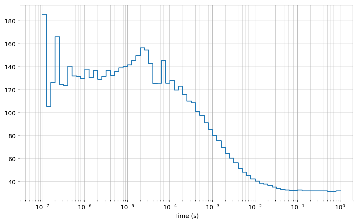
Log-scale bins (base 10)¶

Here we compute the cross-correlation on log10-spaced bins.

First we compute the array of lag bins using the function make_loglags:

In [10]:

# compute lags in sec. then convert to timestamp units
bins = pyc.make_loglags(-7, 0, 10, return_int=False) / unit

Then, we compute the cross-correlation using the function pcorrelate:

In [11]:

G = pyc.pcorrelate(t, u, bins)

/home/docs/checkouts/readthedocs.org/user_builds/pycorrelate/conda/latest/lib/python3.6/importlib/_bootstrap.py:219: RuntimeWarning: numpy.dtype size changed, may indicate binary incompatibility. Expected 96, got 88
  return f(*args, **kwds)

In [12]:

fig, ax = plt.subplots(figsize=(10, 6))
plt.plot(bins*unit, np.hstack((G[:1], G)), drawstyle='steps-pre')
plt.xlabel('Time (s)')
#for x in bins[1:]: plt.axvline(x*unit, lw=0.2)  # to mark bins
plt.grid(True); plt.grid(True, which='minor', lw=0.3)
plt.xscale('log')
plt.xlim(30e-9, 2)

Out[12]:

(3e-08, 2)

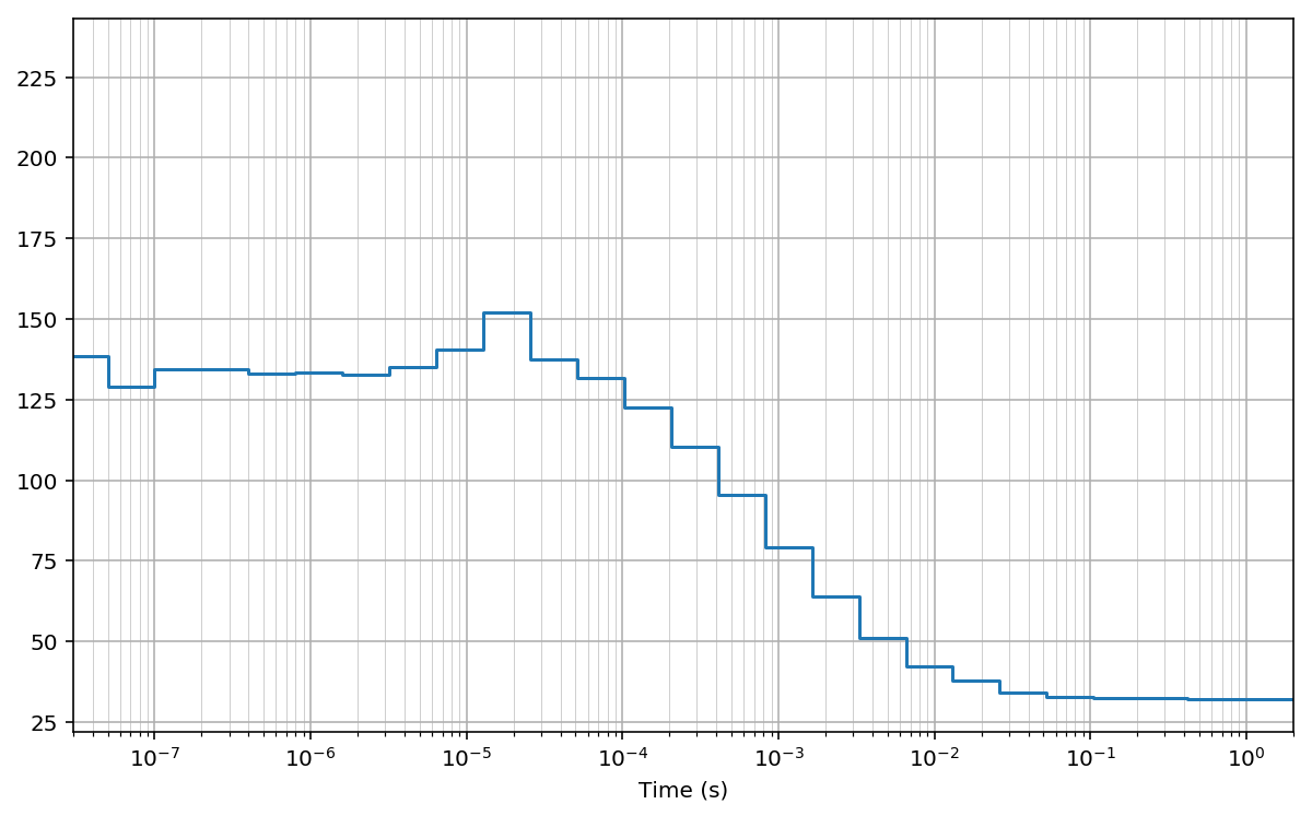
../_images/notebooks_pycorrelate-examples_17_1.png

Log-scale bins (base 2)¶

Here we compute the same cross-correlation on log2-spaced bins.

First we compute the array of lag bins using the function make_loglags:

In [13]:

# compute lags directly in timestamp units
bins = pyc.make_loglags(0, 28, 1, base=2)

Then, we compute the cross-correlation using the function pcorrelate:

In [14]:

G = pyc.pcorrelate(t, u, bins)

In [15]:

fig, ax = plt.subplots(figsize=(10, 6))
plt.plot(bins*unit, np.hstack((G[:1], G)), drawstyle='steps-pre')
plt.xlabel('Time (s)')
#for x in bins[1:]: plt.axvline(x*unit, lw=0.2)  # to mark bins
plt.grid(True); plt.grid(True, which='minor', lw=0.3)
plt.xscale('log')
plt.xlim(30e-9, 2)

Out[15]:

(3e-08, 2)

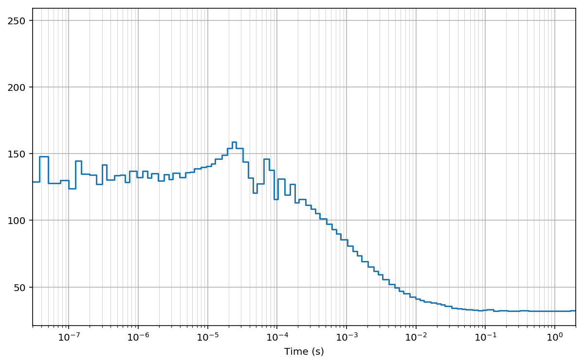
../_images/notebooks_pycorrelate-examples_22_1.png

Multi-tau bins¶

Finally, we compute the cross-correlation on arbitrarly-spaced bins. Similar to the multi-tau bins, here we use constant bin size for a number of bins (n_group), then we double the bin size and we keep it constant for another n_group and so on:

In [16]:

n_group = 4
bin_widths = []
for i in range(26):
    bin_widths += [2**i]*n_group
np.array(bin_widths)
bins = np.hstack(([0], np.cumsum(bin_widths)))

Then, we compute the cross-correlation using the function pcorrelate:

In [17]:

G = pyc.pcorrelate(t, u, bins)

In [18]:

fig, ax = plt.subplots(figsize=(10, 6))
plt.plot(bins*unit, np.hstack((G[:1], G)), drawstyle='steps-pre')
plt.xlabel('Time (s)')
#for x in bins[1:]: plt.axvline(x*unit, lw=0.2)  # to mark bins
plt.grid(True); plt.grid(True, which='minor', lw=0.3)
plt.xscale('log')
plt.xlim(30e-9, 2)

Out[18]:

(3e-08, 2)

../_images/notebooks_pycorrelate-examples_27_1.png

Test: comparison with np.histogram¶

For testing alternative (slower) implementations we use smaller input arrays:

In [19]:

tt = t[:5000]
uu = u[:5000]

The algoritm implemented in pycorrelate.pcorrelate can be re-written in a very simple way using numpy.histogram:

In [20]:

# compute lags in sec. then convert to timestamp units
bins = pyc.make_loglags(-7, 0, 10, return_int=False) / unit

In [21]:

Y = np.zeros(bins.size - 1, dtype=np.int64)
for ti in tt:
    Yc, _ = np.histogram(uu - ti, bins=bins)
    Y += Yc
G = Y / np.diff(bins)

In [22]:

assert (G == pyc.pcorrelate(tt, uu, bins)).all()

Test passed! Here we demonstrated that the logic of the algorithm is implemented as described in the paper (and in the few lines of code above).

Tests: comparison with np.correlate¶

The comparison with np.correlate is a little tricky. First we need to bin our input to create timetraces that can be correlated by linear convolution. For testing purposes, let’s use a small portion of the timetraces:

In [23]:

binwidth = 50e-6
bins_tt = np.arange(0, tt.max()*unit, binwidth) / unit
bins_uu = np.arange(0, uu.max()*unit, binwidth) / unit

In [24]:

bins_tt.max()*unit, bins_tt.size

Out[24]:

(4.13725, 82746)

In [25]:

bins_uu.max()*unit, bins_uu.size

Out[25]:

(1.8020999999999998, 36043)

In [26]:

tx, _ = np.histogram(tt, bins=bins_tt)
ux, _ = np.histogram(uu, bins=bins_uu)

plt.figure(figsize=(10, 6))
plt.plot(bins_tt[1:]*unit, tx)
plt.plot(bins_uu[1:]*unit, ux)
plt.xlabel('Time (s)')

Out[26]:

Text(0.5,0,'Time (s)')

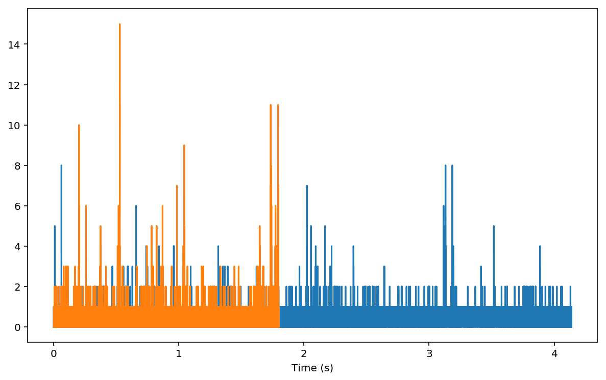
../_images/notebooks_pycorrelate-examples_39_1.png

The plots above are the two curves we are going to feed to np.correlate:

In [27]:

C = np.correlate(ux, tx, mode='full')

We need to trim the result to obtain a proper alignment with the 0-time lag:

In [28]:

Gn = C[tx.size-1:]  # trim to positive time lags

Now, we can check that both numpy.correlate and pycorrelate.ucorrelate give the same result:

In [29]:

Gu = pyc.ucorrelate(tx, ux)
assert (Gu == Gn).all()

Now, let’s compute the correlation also with pycorrelate.pcorrelate:

In [30]:

maxlag_sec = 3.9
lagbins = (np.arange(0, maxlag_sec, binwidth) / unit).astype('int64')

In [31]:

Gp = pyc.pcorrelate(tt, uu, lagbins) * int(binwidth / unit)

Let’s plot a comparison:

In [32]:

fig, ax = plt.subplots(figsize=(10, 6))
Gn_t = np.arange(1, Gn.size+1) * binwidth * 1e3
Gu_t = np.arange(1, Gu.size+1) * binwidth * 1e3
Gp_t = lagbins[1:] * unit * 1e3
plt.plot(Gn_t, Gn, alpha=1, lw=2, label='numpy.correlate')
plt.plot(Gu_t, Gu, alpha=0.6, lw=2, label='pycorrelate.ucorrelate')
plt.plot(Gp_t, Gp, alpha=0.7, lw=2, label='pycorrelate.pcorrelate')
plt.xlabel('Time (ms)', fontsize='large')
plt.grid(True)
plt.xlim(30e-3, 500)
plt.xscale('log')
plt.title('pycorrelate.correlate vs numpy.correlate', fontsize='x-large')
plt.legend(loc='best', fontsize='x-large');

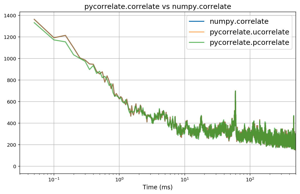
../_images/notebooks_pycorrelate-examples_50_0.png

Conclusion¶

numpy.correlate and pycorrelate.ucorrelate give identical results, with the latter being much faster. Note that the inputs are swapped between the two functions.
pycorrelate.ucorrelate and pycorrelate.pcorrelate agree when using uniform time-lag bins.